Lab2 - dsPIC® MAC Instructions
Objective
The purpose of this exercise is to reinforce understanding of the dsPIC® Multiply-Accumulate (MAC) class instructions by examining an example of their use. We will be applying a second-order polynomial to the averaged result of summing two arrays by using MAC instructions.
Theory of Operation

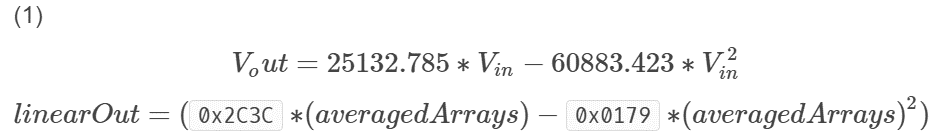
Many types of measurement sensors do not provide a linear output. An example of this is a typical thermocouple system. Fortunately, these outputs can be linearized by use of standard polynomials. These polynomials and their coefficients are provided by the sensor vendor as well as other sources. For this exercise, we use the following standard polynomial from the “Thermal Linear Intelligent Sensor PICtail™ Plus Demo Board User Guide”:
Software Tools
| Tool | About | Installers |
Installation
Instructions |
||
|---|---|---|---|---|---|
| Windows | Linux | Mac OSX | |||
|
MPLAB® X
Integrated Development Environment |
| | | | |
|
MPLAB® XC16
C Compiler |
| | | | |
Exercise Files
| File | Download |
Installation
Instructions |
||
|---|---|---|---|---|
| Windows | Linux | Mac OSX | ||
|
Project and Source Files
|
| | | |
Procedure
Open Project
Start MPLAB® X IDE, then click on the Open Project icon on the main toolbar.
Navigate to the folder where you have saved the downloaded files.
Click on the Lab02.X folder.
Select Open Project .
.
Debug Project
Click on the Debug Project button. This builds and sends the program to the simulator. Click on the Halt
  button. This stops execution so that we may analyze the code.
What just happened?
We took a pre-configured MPLAB X IDE project, which included a complete program, (both C and assembly files included) along with the configuration settings for the tools, and compiled the code contained in the project. After compiling the code, we ran it in the simulator that is built into MPLAB X IDE. (The simulator is capable of reproducing almost all of the functions of a PIC® microcontroller.)
Using DSP accumulator-based operations, the code performs the steps listed below:
a
Populates arrayA[] with 64 values
arrayA[i] = 0x0100 + (rand() & 0x001F);
In this step, we are generating 64 random values between 0x0100 and 0x011F (because we have added a pseudo-random integral number in the range between 0 and 0x001F to our original 0x0100).
b
Populates arrayB[] with 64 values
arrayB[i] = 0x0040 + (rand() & 0x000F);
In this step, we are generating 64 random values between 0x0040 and 0x004F (because we have added a pseudo-random integral number in the range between 0 and 0x000F to our original 0x0040).
c
After we have populated our arrays, we need to pass those parameters from C to assembly. The C functions pass their parameters to other functions (including assembly functions) through the W registers. It is important to note that the W registers are used in the order that the parameters are passed to the function.
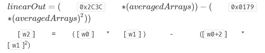
In order to be able to pass both coefficients to just one W register (W0), we created an array of 2 elements called coeffs. As we can see in the code above, the parameter coeffs in the linearize function doesn't need the '&' symbol (which indicates we are passing an address) because C automatically passes the address of the first element inside an array. To access the second coefficient we then just increment W0 as can be seen below:
- Passed to linearize.S:
- W0 : polynomial coefficient a1
- W0+2 : polynomial coefficient a2
- W1 : pointer to averagedArrays
- Returned from linearize.S:
- W2 : pointer to linearOut
d
In the assembly code below, we can observe that the first step is to PUSH our registers onto the stack. Then, after configuring accumulators A and B, we move the addresses of coefficients a1 and a2 into W8 and W9 respectively. Lastly, we move the address of averagedArrays into W10 which is a pointer to Y data space.
e
To calculate the first part of the linearization, we clear Accumulator A, preload W4 with a1, and pre-load W5 with averagedArrays, all in a single instruction. After that, using the MPY instruction, we multiply a1 with averagedArrays and store the result in Accumulator A.
For the second part of the linearization, we first need to square averagedArrays. To do this, we will multiply W5 by W5 since averagedArrays was previously loaded into this register, and store the result in Accumulator B. During that same MPY instruction we are also going to pre-load W4 with the second coefficient, a2. The next step is to store averagedArrays2 into W5.
Lastly, in line 38, we multiply a2 by averagedArrays2 and subtract that from Accumulator A, which previously contained the result of multiplying a1 and averagedArrays together. That result gets stored back into ACCA. Line 42 then stores the result in Accumulator A into W2 which points to the function linearOut.
Results
To be able to see the results of this lab you will have to follow these steps:
Open the Watches Window
 and halting it , open the Watches window by going to Window > Debugging > Watches or by pressing Alt+Shift+2.

In addition to arrayA, arrayB and averagedArrays which you used in Exercise 1, add the linearOut watch to the Watches window.

Place a breakpoint on line 20 in the main.c file. To set a breakpoint, click on the line number where you wish to place the breakpoint.

 button to continue running the debug session. You will notice the program will stop at line 20. At this point, the linearOut watch will display the final result. You can also click on the plus signs next to arrayA and arrayB to see all their elements. (Keep in mind results will be different every time since we are using the rand function.)